# from brainlit.utils import upload, session
# from pathlib import Path
# import napari
# from napari.utils import nbscreenshot
# import os
# %gui qt

/Users/thomasathey/Documents/mimlab/mouselight/env/lib/python3.8/site-packages/python_jsonschema_objects/__init__.py:50: UserWarning: Schema version http://json-schema.org/draft-04/schema not recognized. Some keywords and features may not be supported.
  warnings.warn(

Uploading Brain Images from data in the Octree format.

This notebook demonstrates uploading the 2 lowest-resolution brain volumes and a .swc segment file. The upload destination could easily be set to a url of a cloud data server such as s3.

1) Define variables.

• source and source_segments are the root directories of the octree-formatted data and swc files.

• p is the prefix string. file:// indicates a filepath, while s3:// or gc:// indicate URLs.

• dest and dest_segments are the destinations for the uploads (in this case, filepaths).

• num_res denotes the number of resolutions to upload.

The below paths lead to sample data in the NDD Repo. Alter the below path definitions to point to your own local file locations.

# source = (Path().resolve().parents[2] / "data" / "data_octree").as_posix()
# dest = (Path().resolve().parents[2] / "data" / "upload").as_uri()
# dest_segments = (Path().resolve().parents[2] / "data" / "upload_segments").as_uri()
# dest_annotation = (Path().resolve().parents[2] / "data" / "upload_annotation").as_uri()
# num_res = 2

2) Upload the image data (.tif)

If the upload fails with the error: timed out on a chunk on layer index 0. moving on to the next step of pipeline, re-run the upload_volumes function but with the continue_upload parameter, which takes layer index (the layer index said in the error message) and image index (the last succesful image that uploaded).

For example, if the output failed after image 19, then run upload.upload_volumes(source, dest, num_res, continue_upload = (0, 19)). Repeat this till all of the upload is complete.

# upload.upload_volumes(source, dest, num_res)

Creating precomputed volume at layer index 0: 100%|██████████| 1/1 [00:04<00:00,  4.27s/it]
Creating precomputed volume at layer index 1:   0%|          | 0/8 [00:00<?, ?it/s]
Finished layer index 0, took 4.266659259796143 seconds
Creating precomputed volume at layer index 1: 100%|██████████| 8/8 [00:09<00:00,  1.19s/it]
Finished layer index 1, took 9.484457015991211 seconds

3) Upload the segmentation data (.swc)

If uploading a .swc file associated with a brain volume, then use upload.py. Otherwise if uploading swc files with different name formats, use upload_benchmarking.py

# upload.upload_segments(source, dest_segments, num_res)

converting swcs to neuroglancer format...: 100%|██████████| 1/1 [00:00<00:00, 43.32it/s]
Uploading: 100%|██████████| 1/1 [00:00<00:00, 194.74it/s]

Download the data with NeuroglancerSession and generate labels.

# %%capture
# sess = session.NeuroglancerSession(url=dest, url_segments=dest_segments, mip=0)  # create session object object
# img, bounds, vertices = sess.pull_vertex_list(2, range(250, 350), expand=True)  # get image containing some data
# labels = sess.create_tubes(2, bounds, radius=1)  # generate labels via tube segmentation

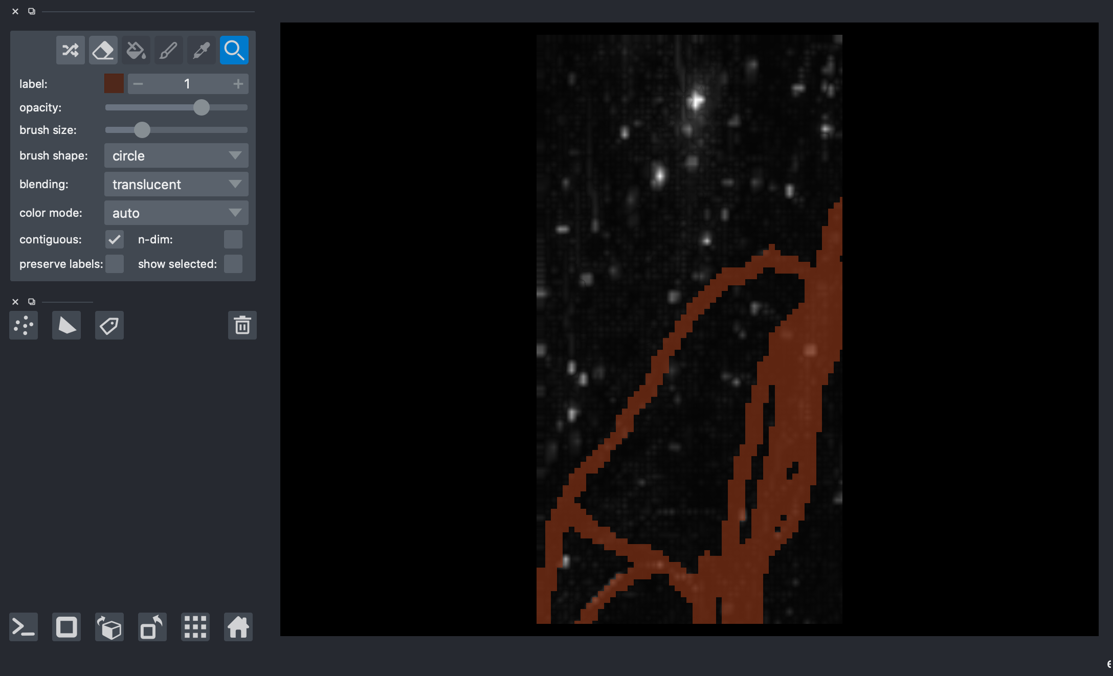
4) Visualize the data with napari

# viewer = napari.Viewer(ndisplay=3)
# viewer.add_image(img)
# viewer.add_labels(labels)
# nbscreenshot(viewer)